Example 4 - Simplistic Runoff Generation
Contents
Example 4 - Simplistic Runoff Generation#
This example illustrates a simple rainfall-runoff generation model
Objective#
This example is to illustrate rainfall-runoff generation in SWMM. The example uses a Horton infiltration excess model, paramaterized so that the %-impervious input in the subcatchment description functions as a runoff coefficient (as in the Rational Equation model)
Note
At the time of writing this vingette, SWMM has no explicit rational method for runoff generation. The runoff generation is via Horton, Green-Ampt, or Curve Number. However if the rational method is appropriate SWMM is probably overkill for the situation - here it is presented as a simplisitc example to illustrate the hydrologic components in SWMM.
Background#
The SWMM program has five runoff generation models built-in: Horton’s Model, Modified Horton’s Model, Green-Ampt Model, Modified Green-Ampt Model and the SCS Curve Number model. The OPTIONS/GENERAL dialog box, listing these four runoff generation (infiltration) options is shown below:
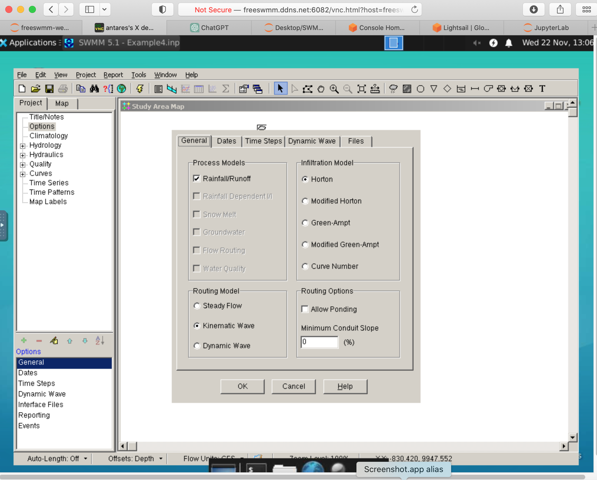
The rational runoff model is not a distinct option; probably the intent is that such flows would be added at individual nodes (which is certainly a legitimate option). However, adjustment of the infiltration model parameters and use of the percent-impervious value allows one to approximate rational runoff behavior directly.
Situation#
Suppose we want to simulate a 10.9 acre drainage area, with \(T_c\) = 49 minutes, and C=0.32 and applied rain depth is 0.87 inches.
The rational method predicts the peak discharge first by determining the precipitation intensity:
\(I = \frac{0.87~\text{inches}}{49~\text{min}} \times 60 \frac{min}{hr} = 1.06 \frac{in}{hr}\)
Then by application of the rational equation:
\(Q_p = (0.32)(1.06)(10.9) = 3.7~ \text{cfs}\)
To produce an equivalent SWMM model as a minimum we need:
Raingage
Catchment
Outlet
We build the model, then adjust some catchment parameters (slope, and width) to match response time (\(T_c\) above) and percent impervious to serve as the runoff coefficient.
Note
A use of this approach might be to replicate an older hydrologic design (such as highway runoff calculations) and then route those flows into a new drainage system that is to be built to support infrastructure expansion. SWMM is actually a good tool to inform such design, but still have to demonstrate it can replicate the pre-development hydrology used in the older design.
To build our model, we need to create a raingage and parameterize it with a constant intensity storm of 1.06 inches per hour.
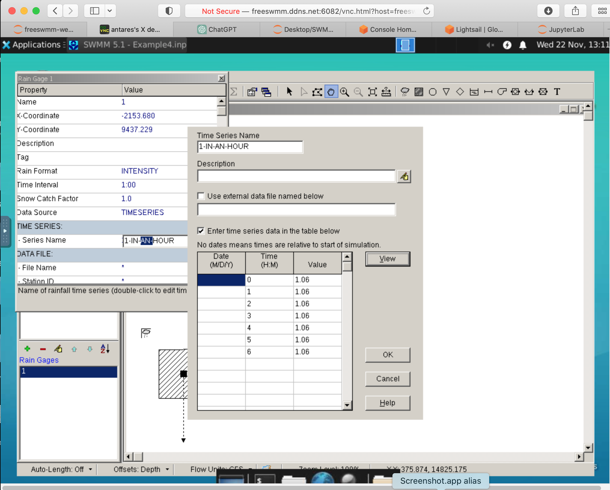
Here we apply the storm for 6 hours - the \(T_c\) is the time to equilibrium in our SWMM model, so we need the storm to be long enough to get to equilibrium; later on we can revert to more meaningful design storms.
Next we parameterize a subcatchment that has area 10.9 acres.
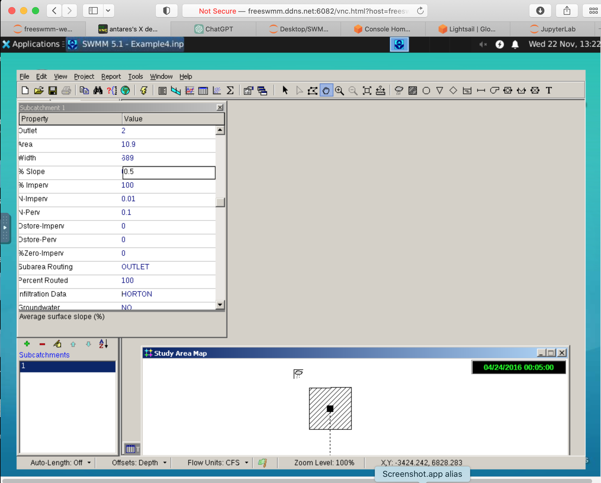
Notice the %-impervious is set to 100 (C=1.0) and the width is 689 feet (the square root of the area) as a starting point. We will use this width to adjust the arrival time of the equilibrium discharge leaving the subcatchmant, then switch the %-impervious to correspond to the supplied value. A lot of the defaults are set to zero as they are not relevant for this example.
The infiltration model used is Horton’s model with the minimum and maximum rates set above the constant intensity so any pervious area absorbs all the precipitation applied, thus letting us use the \5-impervious as a runoff coefficient.
Now we run a simulation and examine the runoff table:
It looks like about 65 minutes elapses until the runoff is the anticipated constant value, so we may need to reduce the response time - enlarging the width will accomplish this task.
Proceeding forward simply change the %-impervious to the prescribed 0.32
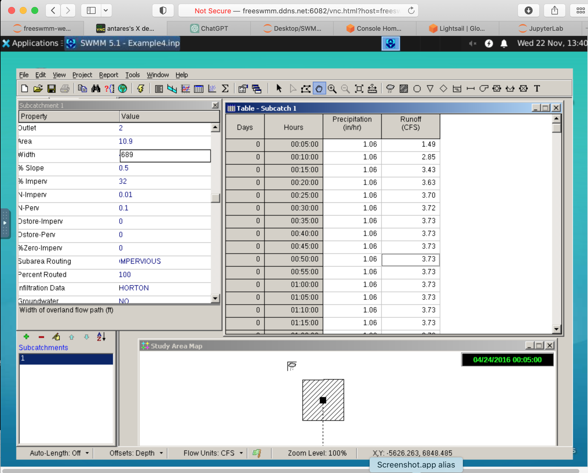
Here we have about 35 minutes until equilibrium, so some adjustment of width is in order; changing to 389 gets the time to equilibrium between 45 and 50 minutes. Close to our target time of 49 minutes (and probably good enough).

The completed data file is linked below.
Supporting Data Files#
This example uses a single input file linked below. There is no background image.
Example4.inp The ASCII input file for this problem.
Using FreeSWMM
Recall the connection starts with a NoVNC interface, then login using freeswmm as the password. Next when the XFCE desktop renders, choose Applications in upper left corner, select WINE in the pull-down menu, then navigate to SWMM 5.1 to start SWMM. All preconfigured examples are accessed using the same procedure.
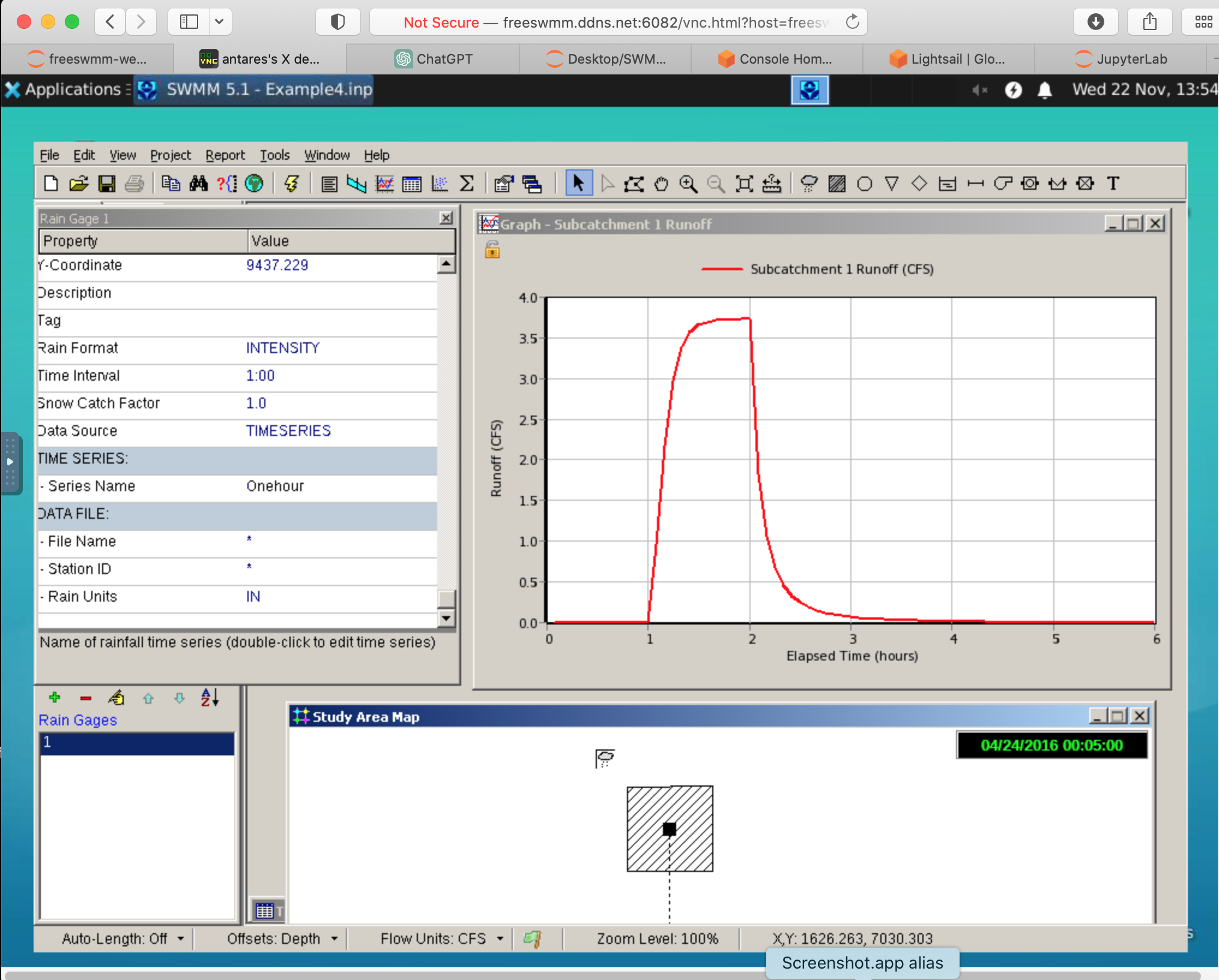
Simulation Results#
The simultion results are shown above, suppose we want to examine a storm that is only an hour long (rather than the 6 hour adjustment storm. We simply modify the rain gage a bit and run and plot as shown below.