Example 3 - GVF Approximation
Contents
Example 3 - GVF Approximation#
While SWMM was not explicitly designed to compute water surface profiles in the classical sense, however it can be coerced to do so using dynamic routing, constant inputs, and running a transient simulation long enough (in simulation time) to reach an equilibrium result which provides a good approximation of gradually varied flow
Objective#
This example is to illustrate the computation and rendering of a water surface profile in an open channel. While SWMM would not be the usual tool for such an exercise, it is certainly capable of the requesite computations.
Situation#
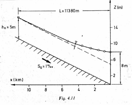
The figure below is a backwater curve for a rectangular channel with discharge over a weir (on the right hand side — not depicted).The channel width is 5 meters, bottom slope 0.001, Manning’s n = 0.02 and discharge Q = 55.4\(\frac{m^3}{s}\).

Note
The figure is from: Page 85. Koutitas, C.G. (1983). Elements of Computational Hydraulics. Pentech Press, London 138p. ISBN 0-7273-0503-4
Our goal is to replicate the figure using SWMM.
Supporting Data Files#
This example uses a single input file linked below - the backdrop is linked as well
example03.inp The ASCII input file for this problem.
bw_curve1.jpg The backdrop image (optional) for this problem.
Below we can connect to FreeSWMM to access the pre-configured file and backdrop.
Using FreeSWMM
Recall the connection starts with a NoVNC interface, then login using freeswmm as the password. Next when the XFCE desktop renders, choose Applications in upper left corner, select WINE in the pull-down menu, then navigate to SWMM 5.1 to start SWMM. All preconfigured examples are accessed using the same procedure.
Selecting the input file#
There is only one .INP file in the pre-placed directory!
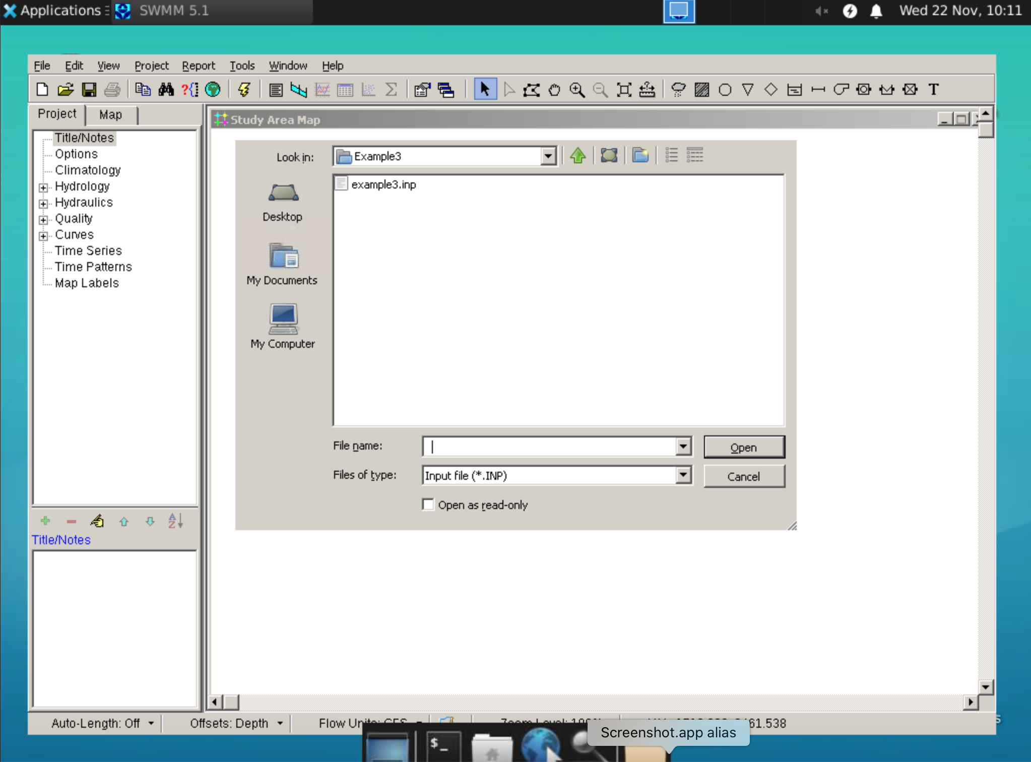
Next load the backdrop if it does not automatically load; then build the model.
Key elements are:
Outfall is a fixed stage outlet, set at 8 meters. Invert is 0 meters.
Each node is an ordinary node; elevations obtained by multiplying node distance from the outfall by 0.001 (the channel slope). These elevations are stored as invert elevations at each node.
Each link is an open rectangular conduit element (choose from pisture menu in interface) with width set to 5 meters, and max depth set to 10 meters (should be enough in this example); Manning’s n is set to 0.02.
The most upstream node (left-most in drwaing canvass) is set to have an inflow value of 55.4 cms.
The simulation time is set to 6 hours (which might be ambitious for an 11 kilometer channel to reach equilibrium - in this case it works fine); Dynamic Wave routing is selected; program defaults work fine in this example, but when seeking an equilibrium solution choosing “Dampen Inertia” terms seems to keep the solution stable - the user has to know when things are at equilibrium, and increase time as needed.
Once everything is set the layout looks something like the figure below:
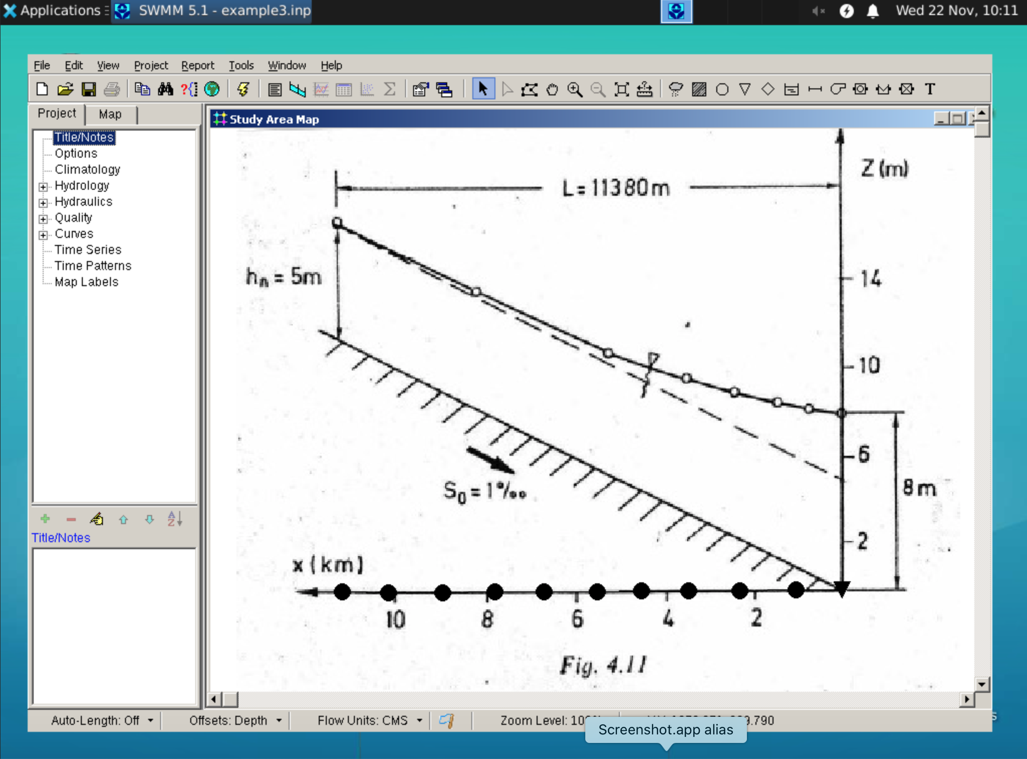
The modeler may want to follow the bottom of the channel in the backdrop - its really user preference at this point. A plan-view map would be pretty dull for this example.
Simulation Results#
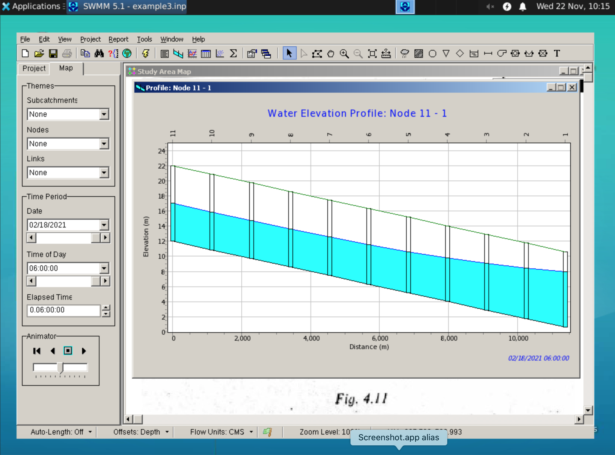
Upon completion of the simulation run (assuming errors and warnings are adresses) one can select the profile plot tool to examine what the water surface profile looks like. Select start node as the upstream node, and end node as the outfall - in this example there is only a single path so the find path search is just fine.
Then in the map tab, move the time slider to the end time - that should be the equilibrium solution; if the user is not sure. Look at the last few time snapshots in the profile - if it is moving about, the model is not yet at equilibrium.
Note
If it is a transient situation, no need to bother with trying to find (a nonexistant) equilibrium result
The result for this example would look something like the image below:
Interpretation#
This example illustrated computation and rendering of a water surface profile in an open channel.
Note
The interested user could instruct SWMM to report the water surface elevations at each node in a table, along with positions then plot these two series onto the backdrop image at the correct aspect ratio - the result would be satisfactory matching.
This plotting would be external to the SWMM program, it takes some fussing to get the aspect ratio correct. A python code fragment to manipulate two images would look something like:
matplotlib.pyplot.rcParams["figure.figsize"] = [10.00, 8.00]
matplotlib.pyplot.rcParams["figure.autolayout"] = True
# read the base image
im = matplotlib.pyplot.imread("Fig5.18.png")
fig, ax = matplotlib.pyplot.subplots()

# set X and Y plot window of basemap
# obtain X,Y values from trial-and-error
im = ax.imshow(im, extent=[-25, 1000, -125, 800])
# then plot the data layer over top of basemap
# adjust X,Y above to get axes to match
References#
Koutitas, C. G. 1983. Elements of Computational Hydraulics. ISBN 0-412-00361-9. Pentech Press Ltd. London. (Chapter 4)
Roberson, J. A., Cassidy, J.J., and Chaudry, M. H., (1988) Hydraulic Engineering, Houghton Mifflin Co (Chapter 10)
Sturm T.W (2001) Open Channel Hydraulics, 1ed., McGraw-Hill, New York. Note: This PDF is from an international edition published in Singapore.
Cunge, J.A., Holly, F.M., Verwey, A. (1980). Practical Aspects of ComputationalRiver Hydraulics. Pittman Publishing Inc. , Boston, MA. pp. 7-50