1.2 Network Hydraulics
Contents
1.2 Network Hydraulics#
Purpose#
This section is a brief overview of the hydraulics of networks to establish a common vocabulary. It assumes some familarity with fluid mechanics and hydraulics, readers can self-teach using the YouTube videos listed in the references.
Pipelines and Networks#
Pipe networks are analyzed for head losses in order to size pumps, determine demand management strategies, and precict minimum pressures in the system.
Pipe Networks#
Network topology refers to the layout and connections.
Networks are built of nodes (junctions) and arcs (links).
Continunity (at a node)#
Water is considered incompressible in steady flow in pipelines and pipe networks, and the conservation of mass reduces to the volumetric flow rate, \(Q\),
\(Q = AV\)
where \(A\) is the cross sectional of the pipe, and \(V\) is the mean section velocity. Typical units for discharge is liters per second (lps), gallons per minute (gpm), cubic meters per second (cms), cubic feet per second (cfs), and million gallons per day (mgd).
The continuity equation in two cross-sections of a pipe as depicted in Fig. 1 is
\( A_1V_1 = A_2V_2 \)
Junctions (nodes) are where two or more pipes join together. A three-pipe junction node with constant external demand is shown in Fig. 2.
The continuity equation for the junction node is

Fig. 1 Continuity of mass (discharge) across a change in cross section#
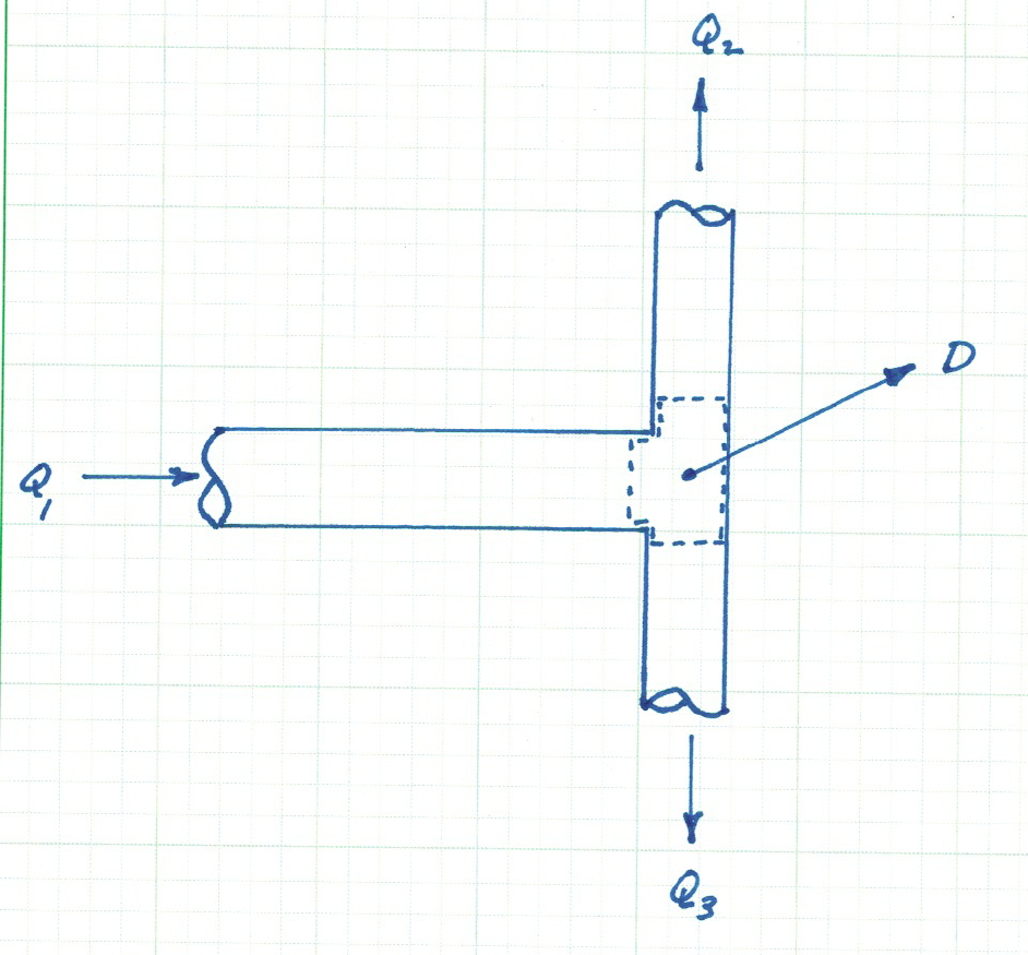
Fig. 2 Continuity of mass (discharge) across a node (junction)#
In a pipe network analysis, all demands on the system are stipulated to be located at junctions (nodes), and the flow connecting junctions is assumed to be uniform across the cross sections (so that mean velocities apply). If a substantial demand is located between nodes, then an additional node is established at the demand location.
For our purposes, a continunity equation is solved for each node in the network to determine heads (or pressures) at that node.
Energy Loss (along a link)#
The equation below is the one-dimensional steady flow form of the energy equation typically applied for pressurized conduit hydraulics.
\( \begin{equation} \frac{p_1}{\rho g}+\alpha_1 \frac{V_1^2}{2g} + z_1 + h_p = \frac{p_2}{\rho g}+\alpha_2 \frac{V_2^2}{2g} + z_2 + h_t + h_f \label{eqn:closed-conduit-energy-equation} \end{equation} \)
where \(\frac{p}{\rho g}\) is the pressure head at a location, \(\alpha \frac{V^2}{2g}\) is the velocity head at a location, \(z\) is the elevation, \(h_p\) is the added head from a pump, \(h_t\) is the added head extracted by a turbine, and \(h_f\) is the frictional head losses between sections 1 and 2. Fig. 3 is a sketch that illustrates the various components in the energy equation.
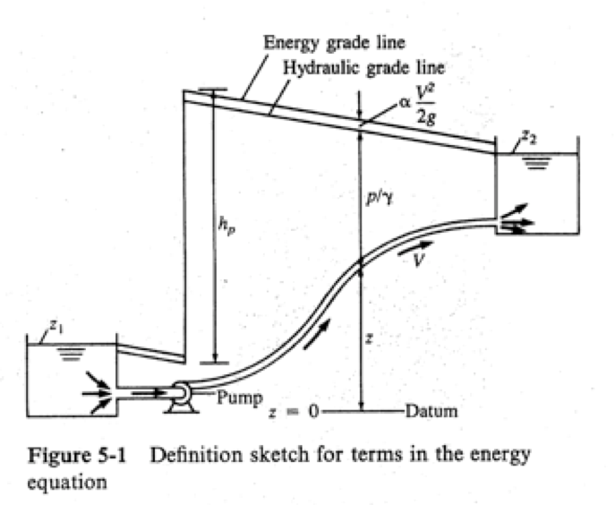
Fig. 3 Definition sketch for energy equation#
In network analysis this energy equation is applied to a link that joins two nodes. Pumps and turbines would be treated as separate components (links) and their hydraulic behavior must be supplied using their respective pump/turbine curves.
For our purposes, an energy equation is solved for each link in the network to determine discharges in that link. If the link is special (a pump or valve) then the appropriate equation is solved for discharge in that special link.
Velocity Head#
The velocity in \(\alpha \frac{V^2}{2g}\) is the mean section velocity and is the ratio of discharge to flow area. The kinetic energy correction coefficient is
\(\begin{equation} \alpha=\frac{\int_A u^3 dA}{V^3 A} \label{eqn:kinetic-energy-correction} \end{equation} \)
where \(u\) is the point velocity in the cross section (usually measured relative to the centerline or the pipe wall; axial symmetry is assumed). Generally values of \(\alpha\) are 2.0 if the flow is laminar, and approach unity (1.0) for turbulent flow. In most water distribution systems the flow is usually turbulent so \(\alpha\) is assumed to be unity and the velocity head is simply \(\frac{V^2}{2g}\).
Added Head — Pumps#
The head supplied by a pump, \(h_p\), is related to the mechanical power supplied to the flow. The relationship of mechanical power to added pump head is
\( \begin{equation} \eta P=Q\rho g h_p \label{eqn:pump-power} \end{equation} \)
where the power supplied to the motor is \(P\) and the “wire-to-water” efficiency is \(\eta\). If the relationship is re-written in terms of added head (negative head loss) the pump curve is
\( \begin{equation} h_p = \frac{\eta P}{Q\rho g} \label{eqn:pump-curve} \end{equation} \)
This relationship stipulates that as discharge increases (for a fixed power) the added head decreases. Power scales at about the cube of discharge, so pump curves for computational application typically have a mathematical structure like
\( \begin{equation} h_p = H_{\text{shutoff}} - K_{\text{pump}}Q^{\text{exponent}} \label{eqn:pump-curve-2} \end{equation} \)
Extracted Head — Turbines#
The head recovered by a turbine is also an “added head” but appears on the loss side of the equation.
The power that can be recovered by a turbine (again using the concept of “water-to-wire” efficiency) is
\( \begin{equation} P=\eta Q\rho g h_t \label{eqn:turbine-power} \end{equation} \)
Head Loss Models#
The Darcy-Weisbach, Chezy-Manning, and Hazen-Williams formulas are relationships between physical pipe characteristics, flow parameters, and head loss. The Darcy-Weisbach formula is the most consistent with the energy equation formulation being derivable (in structural form) from elementary principles (continunity and linear momentum), whereas the other two are empirical (despite the empirical nature of these two models all three are of practical use, and given a choice select your favorite!)
\( \begin{equation} h_{L_f}=f \frac{L}{D} \frac{V^2}{2g} \label{eqn:dw-headloss} \end{equation} \)
where \(h_{L_f}\) is the head loss from pipe friction, \(f\) is a dimensionless friction factor, \(L\) is the pipe length, \(D\) is the pipe characteristic diameter, \(V\) is the mean section velocity, and \(g\) is the gravitational acceleration.
The friction factor, \(f\), is a function of Reynolds number \(Re_D\) and the roughness ratio \(\frac{k_s}{D}\). \( \begin{equation} f=\sigma(Re_D,\frac{k_s}{D}) \label{eqn:friction-factor-dimensionless} \end{equation} \)
The structure of \(\sigma\) is determined experimentally. Over the last century the structure is generally accepted to be one of the following depending on flow conditions and pipe properties
Laminar flow:#
\(\begin{equation} f=\frac{64}{Re_D} \label{eqn:friction-factor-laminar} \end{equation} \)
Hydraulically Smooth Pipes:#
\(\begin{equation} \frac{1}{\sqrt{f}}=-2 log_{10} (\frac{2.51}{Re_d \sqrt{f} }) \label{eqn:friction-factor-smooth} \end{equation} \)
Hydraulically Rough Pipes:#
\( \begin{equation} \frac{1}{\sqrt{f}}=-2 log_{10} (\frac{\frac{k_e}{D}} {3.7}) \label{eqn:friction-factor-rough} \end{equation} \)
Transitional Pipes:#
\( \begin{equation} \frac{1}{\sqrt{f}}=-2 log_{10} (\frac{\frac{k_e}{D}} {3.7} + \frac{2.51}{Re_d \sqrt{f} } ) \label{eqn:friction-factor-CW} \end{equation} \)
Transitional Pipes (Jain Formula):#
\(\begin{equation} f=\frac{0.25}{[log_{10} (\frac{\frac{k_e}{D}} {3.7} + \frac{5.74}{Re_d^{0.9} } )] ^2} \label{eqn:friction-factor-Jain} \end{equation} \)
Emergent work reported in Pomerenk, et al. (2023) provides a unified theory of pipe flow, which may make the above models obsolete.
Pipe Networks Solution Methods#
Several methods are used to produce solutions (estimates of discharge, head loss, and pressure) in a network.
An early one, that only involves analysis of loops is the Hardy-Cross method.
A later one, more efficient, is a Newton-Raphson method that uses node equations to balance discharges and demands, and loop equations to balance head losses. The use of loop equations requires a technique to traverse loops, usually based on graph theory for directed graphs which can be quite complicated for large systems.
However, a rather ingenious method exists developed by Hamam, Y.M., and Brameller, A. (1971), where the flow distribution and head values are determined simultaneously; this is the method used (with some adaptations) within EPANET.
The fundamental procedure is:
Continuity is written at nodes (node equations).
Energy loss (gain) is written along links (pipe equations).
The entire set of equations (non-linear) is solved simultaneously.
An example to illustrate the construction of a pipe network problem follows
Network Analysis Example#
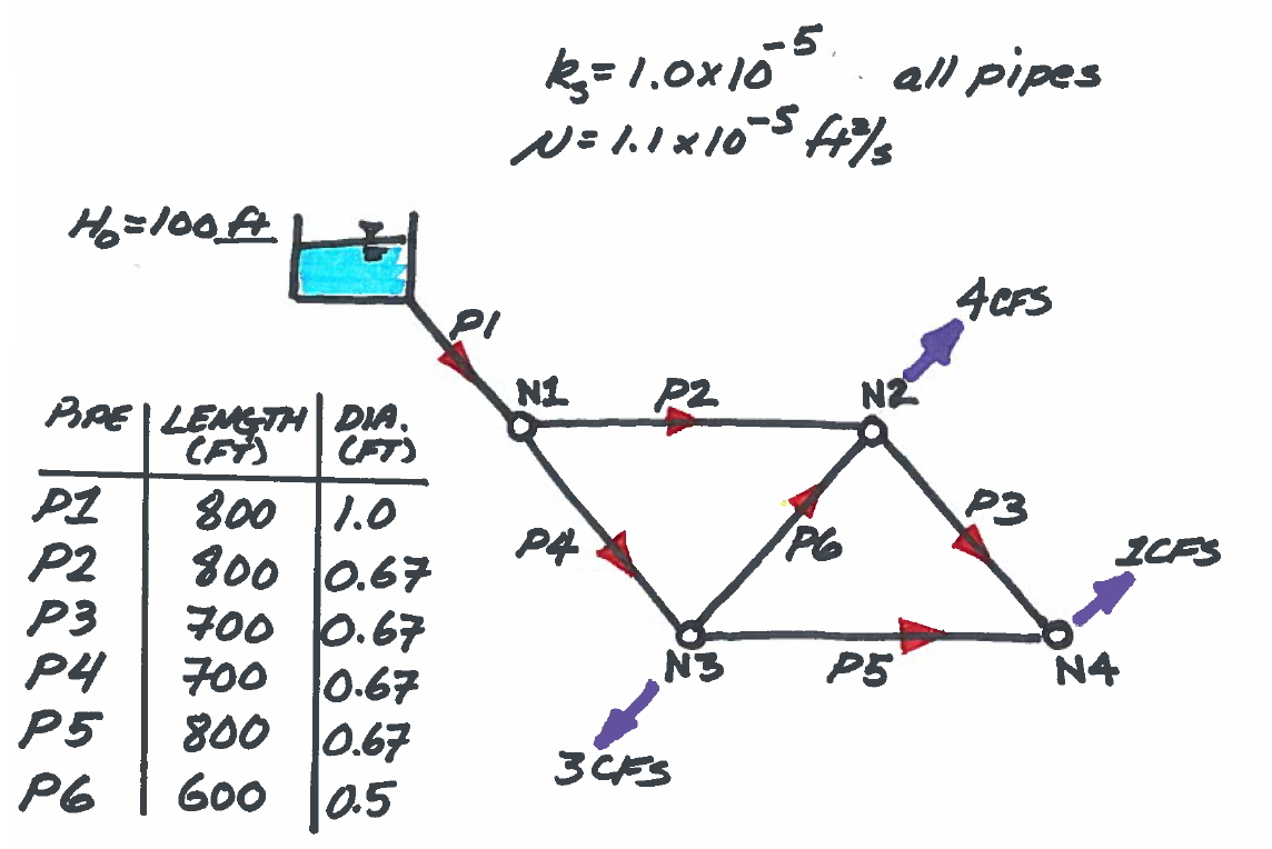
Fig. 4 Pipe network for illustrative example with supply and demands identified. Pipe dimensions and diameters are also depicted.#
Fig. 4 is a sketch of the problem that will be used.
The network supply is the fixed-grade node in the upper left hand corner of the drawing.
The remaining nodes (N1 – N4) have demands specified as the purple outflow arrows.
The pipes are labeled (P1 – P6), and the red arrows indicate a positive flow direction, that is, if the flow is in the indicated direction, the numerical value of flow (or velocity) in that link would be a positive number.
Define the flows in each pipe and the total head at each node as \(Q_i\) and \(H_i\) where the subscript indicates the particular component identification. Expressed as a vector, these unknowns are:
\( \begin{matrix} [Q_1, & Q_2, & Q_3, & Q_4, & Q_5, & Q_6, & H_1, & H_2, & H_3, &H_4 ]& = & \textbf{x} \\ \end{matrix} \)
If we analyze continuity for each node we will have 4 equations (corresponding to each node) for continunity, for instance for Node N2 the equation is
\( \begin{matrix} ~& Q_2 & -Q_3 & ~ & ~ & Q_6 & ~ & ~ & ~ &~ & = & 4\\ \end{matrix} \)
Similarily if we define head loss in any pipe as \(\Delta H_i = f \frac{8 L_i}{\pi^2 g D_i^5} |Q_i| Q_i\) or \(\Delta H_i = L_i Q_i\), where \(L_i = f \frac{8 L_i}{\pi^2 g D_i^5} |Q_i|\), then we have 6 equations (corresponding to each pipe) for energy, for instance for Pipe (P2) the equation is:
\( \begin{matrix} ~& -L_2Q_2& ~ & ~ & ~ & ~& H_1 & -H_2 & ~ & ~ & = & 0\\ \end{matrix} \)
If we now write all the node equations then all the pipe equations we could construct the following coefficient matrix below
Note
The horizontal lines divide the node and the pipe equations.
The upper partition are the node equations in Q and H, the lower partition are the pipe equations in Q and H}
\( \begin{matrix} \hline ~1&-1 & 0 & -1 & 0 & 0 & 0 & 0 & 0 &0 \\ 0&~1 & -1 & 0 & 0 &~1 & 0 & 0 & 0 &0 \\ 0& 0 & 0 &~1 & -1 & -1 & 0 & 0 & 0 &0 \\ 0& 0 &~1 & 0 &~1 & 0 & 0 & 0 & 0 &0 \\ \hline -L_1& 0& 0 & 0 & 0 & 0 & -1 & 0 & 0 &0 \\ 0& -L_2& 0 & 0 & 0 & 0&~1 & -1 & 0 &0 \\ 0& 0& -L_3 & 0 & 0 & 0& 0 &~1 & 0 & -1 \\ 0& 0& 0 & -L_4 & 0 & 0&~1 & 0 & -1 & 0 \\ 0& 0& 0 & 0 & -L_5 & 0& 0 & 0 &~1 & -1 \\ 0& 0& 0 &0 & 0 & -L_6& 0 & -1 &~1 & 0 \\ \hline \end{matrix} \)
Declare the name of this matrix \(\textbf{A(x)}\), where \(\textbf{x}\) denotes the unknown vector of Q augmented by H as above. Next consider the right-hand-side at the correct solution (as of yet still unknown!) as
\( \begin{matrix} [0, & 4, & 3, & 1, & -100 , & 0, & 0, & 0, & 0, &0 ] = \textbf{b}\\ \end{matrix} \)
So if the coefficient matrix is correct then the following system would result: \( \mathbf{A(x)} \cdot \mathbf{x} = \mathbf{b} \)
which would look like
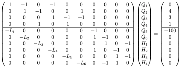
Fig. 5 Pipe network illustrative example as Matrtx-Vector system of equations.#
The solution to the system in Fig. 5 returns the flows in each link and the total heads at each node.
Observe, the system is non-linear because the coefficient matrix depends on the current values of \(Q_i\) for the \(L_i\) terms. However, the system is full-rank (rows == columns) so it is a candidate for Newton-Raphson.
Further observe that the upper partition from column 6 and smaller is simply the node-arc incidence matrix, and the lower partition for the same columns only contains \(L_i\) terms on its diagonal, the remainder is zero. Next observe that the partition associated with heads in the node equations is the zero-matrix.
Lastly (and this is important!) the lower right partition is the transpose of the node-arc incidence matrix subjected to scalar multiplication of \(-1\). The importance is that all the information needed to find a solution is contained in the node-arc incidence matrix and the right-hand-side – the engineer does not need to identify closed loops (nor does the computer need to find closed loops).
The trade-off is a much larger system of equations, however solving large systems is far easier that searching a directed graph to identify closed loops, furthermore we obtain the heads as part of the solution process.
The Newton-Raphson solution method using python is presented later in section 1.4.
References#
Pomerenk, Olivia, et al. “Hydrodynamics of Finite-Length Pipes at Intermediate Reynolds Numbers.” Journal of Fluid Mechanics, vol. 959, 2023, p. A28., doi:10.1017/jfm.2023.99.
